Calibration & the Measurement Run: How the Machine Learns What One Pixel Means

Teardown A4. Cameras speak pixels; motors speak millimeters. Between them sits one scale factor the machine cannot measure with any ruler — so it weighs it out itself. The measurement run, the full pixel-to-motor chain, and why a wrong scale is k arriving through another door. With an interactive coordinate-transform lab.

In A3.5 I quietly cheated: I let the camera report millimeters — Δx = +1.40 mm — and ran straight to the motors. But a camera knows nothing about millimeters. What it actually reports is pixels: “the mark moved from column 512 to column 592.” Meanwhile the motor only accepts millimeters. Between the two sits a conversion, and it is a conversion the machine cannot possibly know at the factory — every lens swap, every mounting-height change rewrites it. Where that conversion comes from is this entire unit.

How Big Is One Pixel, Really?

The camera’s view is a grid of pixels (Figure 1). The mark lands on the grid; the camera counts squares. The question: how many millimeters is one square?

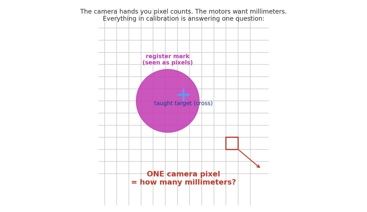
Pixel grid with a register mark and a taught cross; one pixel highlighted with the question: how many millimeters? — Fig. 1 — The camera hands you pixel counts. The motors want millimeters. All of calibration is answering one question: one pixel = how many millimeters?

The answer depends on the lens, the mounting height, the sensor — none of which the machine can reach with a ruler. The ruler lives outside the camera, and the camera is buried under the table. There is exactly one way out: let the machine weigh the factor out by itself. That procedure is the measurement run.

The Measurement Run: Five Beats, None Skipped

The machine holds two assets nobody else has: a motor that can travel a known, exact distance, and a camera that can count pixels exactly. Connect the two and the factor falls out (Figure 2):

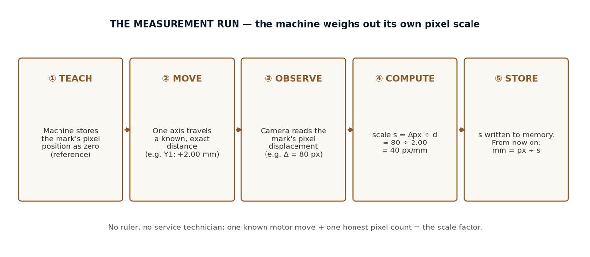
Five-step flow: teach, move a known distance, observe pixel displacement, compute the scale, store it — Fig. 2 — The measurement run: teach → move → observe → compute → store. No ruler, no service technician.

Teach. With the mark correctly positioned, the machine records its pixel position as zero (the reference).
Move. One axis travels a known, exact distance — say Y1: +2.00 mm. This is the ground truth nobody argues with: a servo that goes 2.00 mm went 2.00 mm.
Observe. The camera counts how many pixels the mark shifted — say Δ = 80 px. This is the honest observation: cameras never lie about pixel counts.
Divide. s = Δpx ÷ d = 80 ÷ 2.00 = 40 px/mm. Flipped around: 1 px = 1 ÷ 40 = 0.025 mm.
Store. s goes into memory. From now on: mm = px ÷ s.

A full worked example, every division shown (Figure 3):

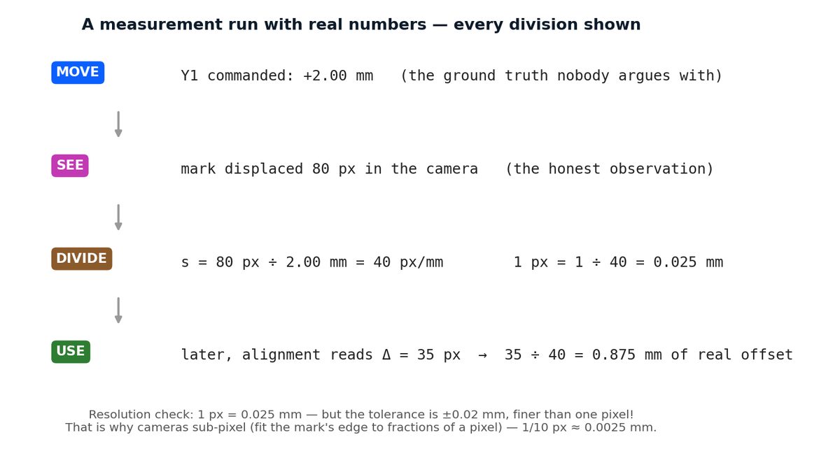
Worked example chain: move 2.00 mm, see 80 px, divide to get 40 px per mm, then use it on a 35 px reading — Fig. 3 — MOVE / SEE / DIVIDE / USE, with real numbers. Later, a 35 px reading becomes 35 ÷ 40 = 0.875 mm of real offset.

A resolution check that should bother you: 1 px = 0.025 mm, but the alignment tolerance is ±0.02 mm — finer than one pixel. That is why these cameras work in sub-pixels: they fit the mark’s edge to a fraction of a pixel, typically around 1/10 px ≈ 0.0025 mm. Sub-pixel fitting is not a luxury here; it is the hard prerequisite for the tolerance.

The Full Conversion: From Pixels to Motor Commands

Every correction round runs one complete address-translation chain (Figure 4):

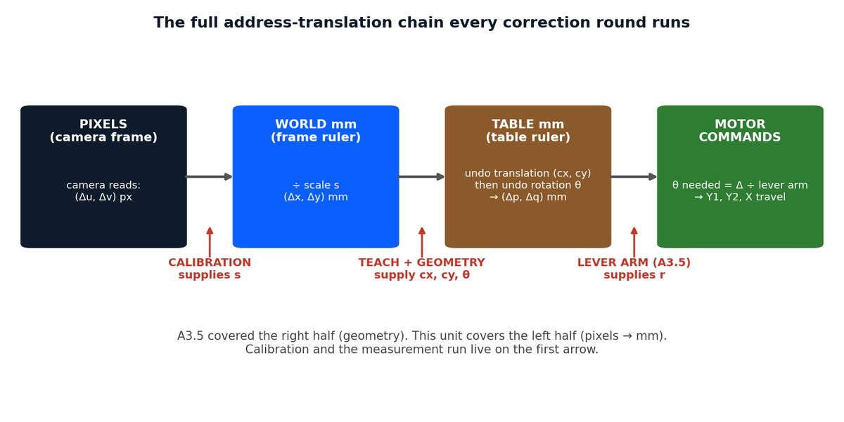
Chain: pixels to world mm to table mm to motor commands, with calibration, teach geometry, and lever arm feeding the three arrows — Fig. 4 — The chain every correction round runs. Calibration supplies s for the first arrow; teach geometry supplies the pose for the second; the lever arm (A3.5) supplies r for the third.

Arrow 1 — pixels → world millimeters. The camera reports (Δu, Δv) px; divide by s to get (Δx, Δy) mm. s comes from calibration — the subject of this unit.

Arrow 2 — world mm → table mm. Between the world ruler (bolted to the frame) and the table ruler (rotating with the table) sit a rotation θ and a translation (cx, cy). To go from world back to table you invert the transform — undo the translation first, then undo the rotation (the order is not optional):

① undo translation:  dx = x − c_x,  dy = y − c_y
② undo rotation (rotate by −θ):
   p = dx·cosθ + dy·sinθ
   q = −dx·sinθ + dy·cosθ

θ, cx and cy come from the geometry recorded at teach time.

Arrow 3 — table mm → motor commands. The needed rotation is θ = Δ ÷ r, distributed across Y1, Y2 and X. r comes from the lever-arm geometry — everything A3.5 was about.

So the chain’s three parameters — s, the pose, and r — are supplied by calibration, teach, and geometry respectively. This unit owns the first arrow; A3.5 owns the third. The middle arrow is exactly what the embedded lab below gives you a feel for.

Try It Yourself: The Coordinate Transform Lab

The lab below is the second arrow made tangible — plus a pixel panel for the first:

Move the table: sliders drive θ, cx, cy directly (one preset reproduces A3.5’s exact worked example — Y1 +2 mm ⇒ θ = −0.1637°). Drag the purple mark: its table address (p, q) never changes; its world address (x, y) changes with every table move.
Forward transform, live: x = p·cosθ − q·sinθ + cx with your current numbers substituted at every step — no multiplication hidden.
And back again: the camera only reads the world ruler, so the controller must invert the transform to compare “where the mark is” with “where it was taught” — translation undone first, then rotation, until the mark’s true identity (p, q) is recovered in front of you.
Where pixels enter: two sliders set the true scale and the stored scale. Line ① of the panel — the pixel count — never lies. Everything after it is the stored scale’s opinion. When the two scales match, the mm reading is exact; when they don’t, the machine computes a wrong displacement with total confidence.

The Full view button expands the lab to fill your screen — much more comfortable on a phone.

When the Stored Scale Is Wrong: k Through Another Door

In A3.5 the convergence factor k = 1 − D_true ÷ D_assumed came from a stale lever arm. Here is the symmetrical story (Figure 5). The camera honestly reports Δ px; the machine believes Δ ÷ s_stored mm; the truth is Δ ÷ s_true mm. So:

belief = truth × (s_true ÷ s_stored)
→ every correction is computed from belief
→ the residual multiplier becomes k = 1 − s_true ÷ s_stored

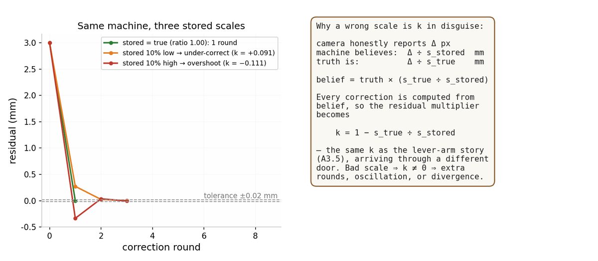
Left: convergence curves for three stored scales; right: the derivation that k = 1 − s_true ÷ s_stored — Fig. 5 — The same k, arriving through a different door. Stored scale 10% low ⇒ k = +0.091, slow under-correcting crawl; 10% high ⇒ k = −0.111, oscillating overshoot; ratio ≥ 2 ⇒ divergence.

The same k, through another door. Which is why calibration runs before alignment, not after: a scale that is off by even a few percent silently taxes every single correction round.

When to Re-Calibrate

Lens swapped, camera nudged, mounting height changed — s is void immediately.
New screen or stock changes how the mark images — the sub-pixel fitting baseline moved.
Alignment suddenly takes extra rounds, or starts swinging left-right — that is k ≠ 0 talking. Suspect the scale first, the lever arm second.

Terms in This Note

Pixel scale (s, px/mm) — the only bridge between camera pixels and real millimeters; the product of the measurement run.
Measurement run — teach zero → move a known distance → count pixels → divide → store.
Sub-pixel fitting — fitting the mark’s edge to a fraction of a pixel (~1/10 px); the hard prerequisite for a ±0.02 mm tolerance.
Forward / inverse transform — table→world (rotate, then translate); world→table (undo translation, then undo rotation).
k’s second door — k = 1 − s_true ÷ s_stored; same shape as the lever-arm version, different cause.

Next in A5: laser positioning — the no-camera alignment option, and the open-loop vs. closed-loop argument.