The Geometry Under Vision Alignment: Pivots, Lever Arms, and the Correction Loop

In A1 we followed one camera aligning one mark, and in A3 we saw how two cameras share a correction. But I kept skating past a harder question: how exactly does the machine turn “the camera sees an offset” into “each axis moves this many millimeters”? I realized I couldn’t truly explain it until I rebuilt the whole chain myself — physics, coordinates, iteration, and all. This note is that rebuild. Nothing here comes from any manual; it is the minimal geometry every camera-registered flatbed press shares, written in plain language with high-school math, plus an interactive lab (embedded below) so you can watch every formula become real numbers.

A Minimal Model of the Whole System

Strip a vision alignment system down to its skeleton and five roles remain (Figure 1):

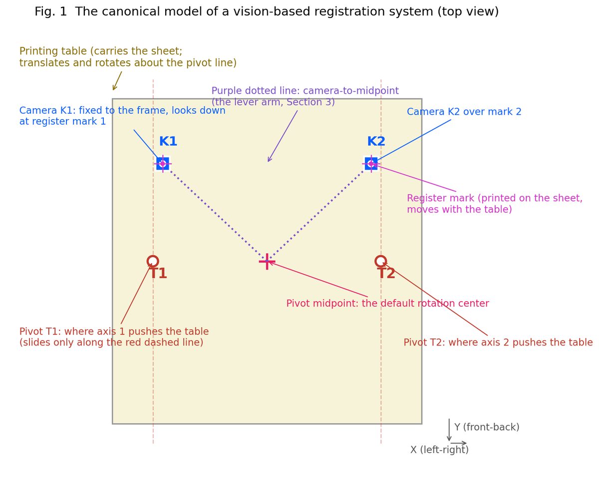
• The table: a rigid plate carrying the sheet. It can shift left-right, front-back, and rotate by a tiny angle.
• Two linear motor axes (Y1, Y2): each pushes the table at one point, strictly along its own front-back axis line. Their spacing is fixed — 700 mm in the examples here.
• Pivots (T1, T2): the contact points where the motors push. When the two axes push unequally, the table must rotate about some point on the line between them.
• Two cameras (K1, K2): bolted to the machine frame, looking straight down, each watching one register mark on the sheet.
• Two marks: reference graphics printed on the sheet, moving with the table.

Add a third axis (X) for left-right motion, and all three in-plane degrees of freedom are under motor control. The whole alignment process in one sentence: the cameras measure how far the marks are off, the machine computes how far each axis should travel, and the offset is removed. The hard part is not the looking — it is the computing. Between “what the camera sees” and “what the motor should do” sits a geometric conversion. Let’s take it apart.

Concept 1: The Pivot and the Center of Rotation

Plain language: two people carry a table. The one on the left walks half a step farther forward — the table rotates, about the right person’s hand. That unmoving hand is the pivot.

In math: axes Y1 and Y2 push at pivots T1 and T2. If in one move Y1 travels y₁ and Y2 travels y₂, a right triangle appears (Figure 2): the adjacent side is the fixed 700 mm pivot spacing, the opposite side is the difference y₂ − y₁.

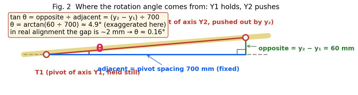
The table’s rotation angle follows from the tangent relation:

With real numbers: if Y2 outruns Y1 by 60 mm, θ = arctan(60 ÷ 700) ≈ 4.9°. In real alignment the difference is more like 2 mm, so θ ≈ 0.16° — a tilt your eye could never catch. But the lever arm (next concept) amplifies that invisible tilt into millimeters the camera cannot miss.

When Y1 retracts and Y2 advances by equal amounts, the only point that doesn’t move is the midpoint of the two pivots — the center of rotation for the symmetric case. Everything below uses the midpoint unless stated otherwise.

Concept 2: The Lever Arm

Plain language: same table, still rotating. Points far from the center of rotation sweep long arcs; points near it barely move. How far the camera “stands” from the center decides how large a displacement any given rotation produces in its view. That distance is the lever arm.

In math: the lever arm r is the in-plane distance from the camera’s aim point to the center of rotation (Figure 3). In-plane, note — the camera’s mounting height plays no role, because it looks straight down and the mark moves within the table plane. With horizontal/vertical offsets Δx and Δy, Pythagoras gives:

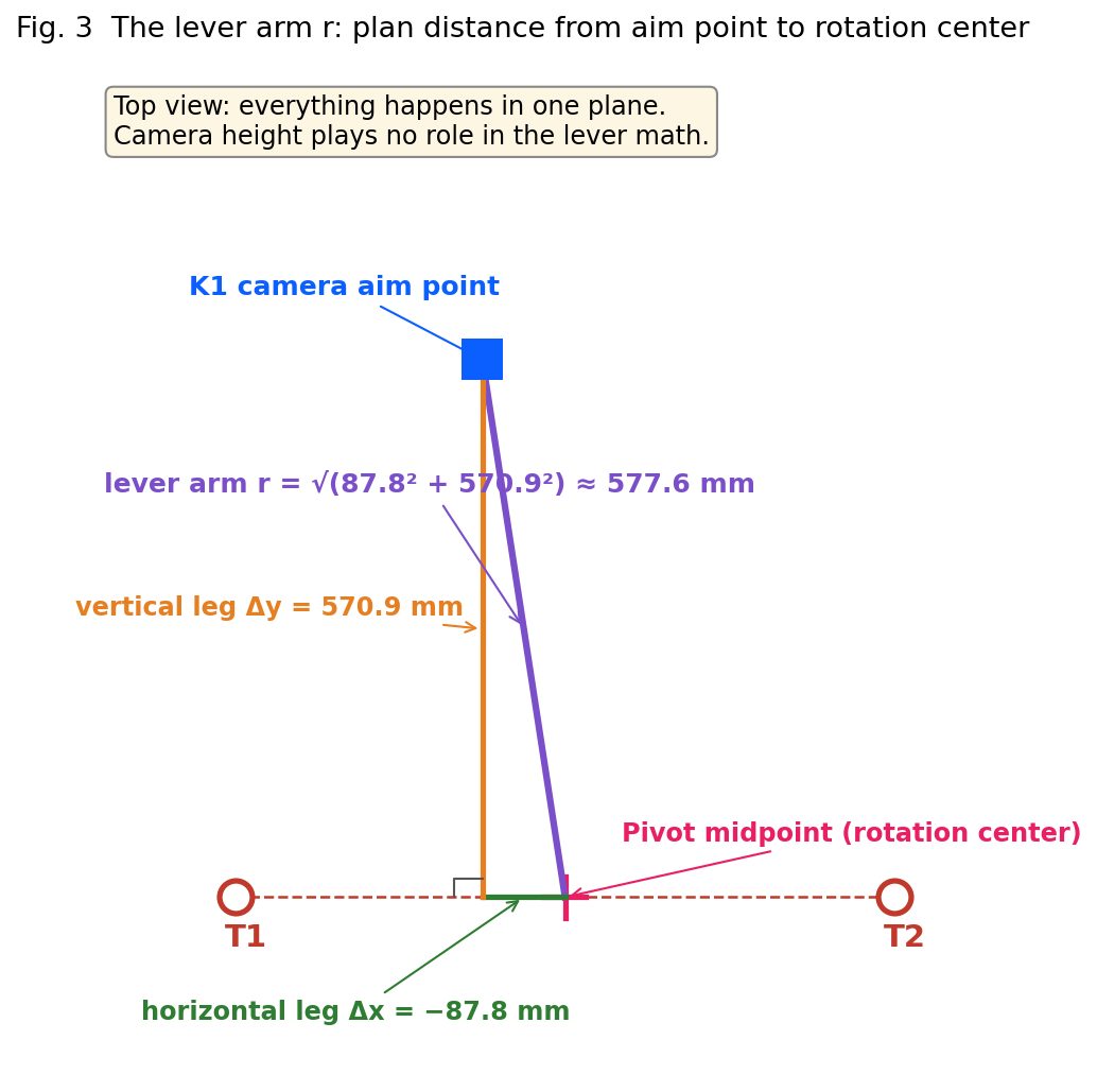
With real numbers: Δx = −87.8 mm, Δy = 570.9 mm → r = √(87.8² + 570.9²) ≈ 577.6 mm.

The lever arm’s job in one sentence: when the table rotates by θ, the mark’s displacement at the camera ≈ θ × r (at small angles the arc is nearly straight). That sentence hides four small steps — here they are, none skipped (Fig. 3b):

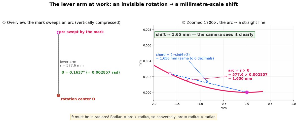
Step 1 — where θ comes from. Y1 moved 2 mm, Y2 stayed: difference 2 mm over a 700 mm pivot spacing, so θ = arctan(2 ÷ 700) = 0.1637°.

Step 2 — degrees to radians: the step everyone skips. Arc-length math needs radians. The radian is disarmingly simple: arc length ÷ radius = angle in radians. A full circle is 360° = 2π rad, so 1° = π ÷ 180 = 0.0174533 rad, and θ = 0.1637 × 0.0174533 = 0.002857 rad.

Step 3 — the mark travels an arc. It sits 577.6 mm from the center of rotation, so θ carries it along an arc of a 577.6 mm-radius circle. Flip the radian definition around: arc = radius × radian = 577.6 × 0.002857 = 1.650 mm.

Step 4 — why the arc may be treated as a straight shift. The camera measures a straight line (the chord), not an arc. Check the difference: chord = 2r × sin(θ ÷ 2) = 2 × 577.6 × sin(0.00142857) = 1.650285 mm — identical to the arc (1.650281 mm) for the first five decimals. “Arc ≈ straight line” is bookkeeping, not laziness.

Bottom line: a 0.1637° rotation your eye could never catch is amplified by the 577.6 mm lever arm into a 1.65 mm shift — the entire secret of how a camera sees micron-scale table rotation.

Concept 3: Table Coordinates vs. World Coordinates

Plain language: there are two rulers. One is nailed to the table and turns with it; the other is nailed to the frame and never moves. A mark is printed on the sheet, so its reading on the first ruler never changes. But the camera lives on the frame — it only reads the second ruler. When the table turns, the same point gets a new reading on the second ruler.

In math (Figure 4): a mark at table coordinates (p, q), with table rotation θ and translation (cx, cy), lands at world coordinates:

This is the rotate-then-translate transform (formally a 2D rotation matrix — don’t fear the word; it’s just the four multipliers cosθ, −sinθ, sinθ, cosθ in a fixed pattern).

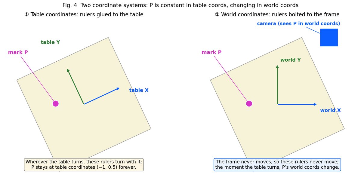
With real numbers: mark at table coords (−320, 300), Y1 moves +2 mm while Y2 stays. Then θ = arctan(−2 ÷ 700) ≈ −0.164°, sin θ ≈ −0.002857, cos θ ≈ 0.999996, and the midpoint translation cy = (2+0)÷2 = 1 mm. Substituting:

• x = (−320)×0.999996 − 300×(−0.002857) + 0 ≈ −319.1
• y = (−320)×(−0.002857) + 300×0.999996 + 1 ≈ +301.9

Look at where the 0.86 mm change in x came from: almost entirely the term −300×sinθ. A point 300 mm from the rotation center in the front-back direction, multiplied by the angle, produces sideways displacement. The lever arm lives inside that product. (This was the single step that took me the longest to internalize — if it looks opaque, open the lab below, press Y1＋ once, and watch this exact arithmetic printed line by line.)

Concept 4: The Deviation Δ

Plain language: the camera view holds a cross and a dot. The cross is where the mark should be — recorded by a teach action during a correctly positioned setup. The dot is where the mark actually is right now. Alignment is the business of erasing the distance from dot to cross.

In math (Figure 5): the deviation Δ is actual minus target:

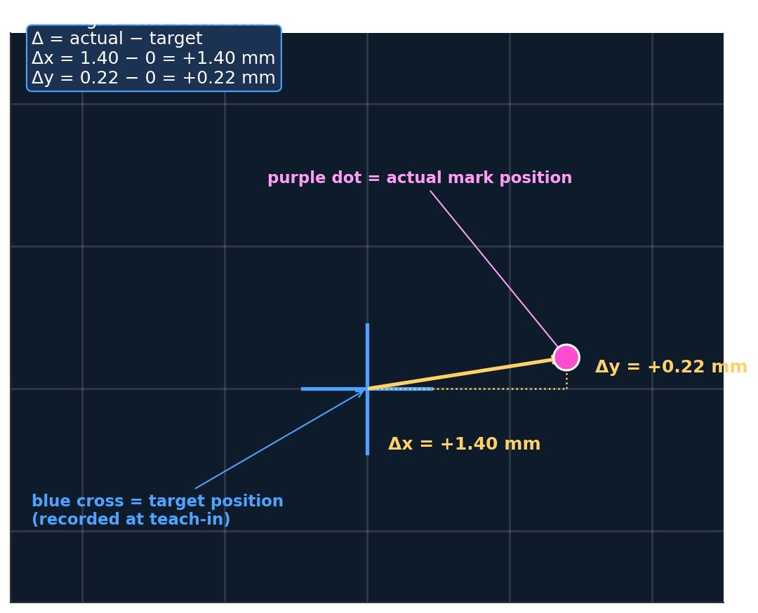
With real numbers: dot at (1.40, 0.22), cross at (0, 0) → Δx = +1.40 mm, Δy = +0.22 mm.

Concept 5: The Convergence Tolerance

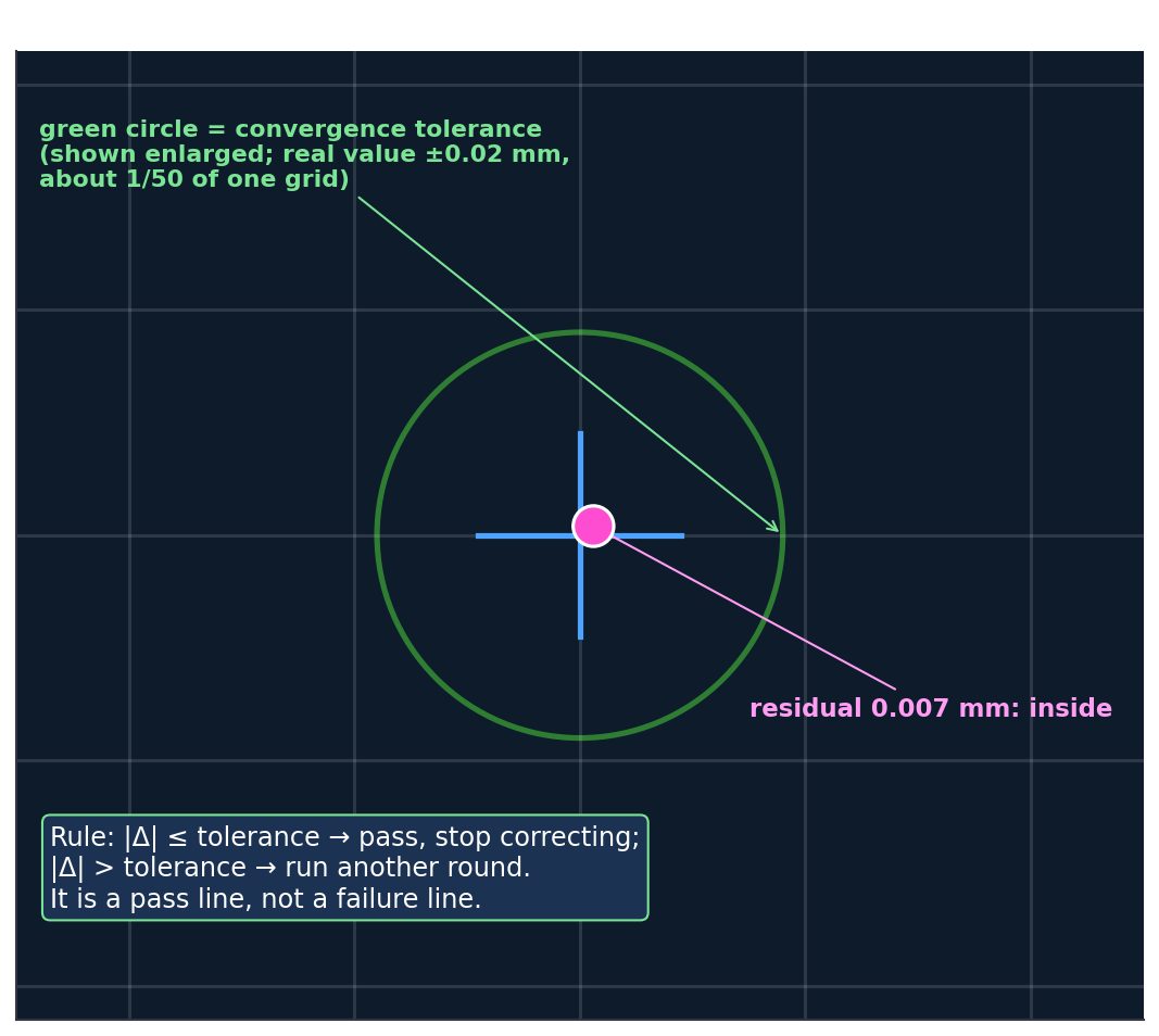
Plain language: “perfectly aligned” does not exist. Motors have a minimum step, cameras have pixel noise, material breathes. The system doesn’t need Δ = 0; it needs Δ small enough. That boundary is the convergence tolerance — a pass line, not a fail line.

In math (Figure 6): with tolerance ε (a typical value is ±0.02 mm), check after every correction round:

The Algorithm: Four Beats per Round

With the five concepts in hand, the complete algorithm is a four-beat loop (Figure 7):

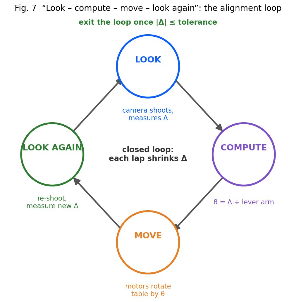
Beat 1 — Look. The camera photographs and measures the deviation. Say Δx = +1.40 mm this round.

Beat 2 — Compute. Translate deviation into angle. Since an angle θ produces displacement θ × r at lever arm r, removing Δ needs θ = Δ ÷ r = 1.40 ÷ 577.6 ≈ 0.00242 rad ≈ 0.139°.

Beat 3 — Move. Translate angle into motor commands. To rotate θ about the pivot midpoint, Y1 and Y2 each travel θ × 350 mm in opposite directions (350 mm = midpoint-to-pivot distance): 0.00242 × 350 ≈ 0.85 mm. So: Y1 +0.85 mm, Y2 −0.85 mm, and the X axis removes the pure translation part of Δ.

Beat 4 — Look again. New picture, new residual. If |Δ| ≤ ε, done; otherwise loop back to beat 1.

Ideally one round suffices. But “ideally” rests on a hidden premise: the lever arm r used in beat 2 must be the true geometry. What if the machine’s stored r is stale — say a camera was nudged during a changeover? That question is the rest of this note.

When the Stored Geometry Is Wrong: Meet k

Start with a shower. The water’s cold, so you nudge the handle toward hot, wait, test — still cold, nudge again. You never crank it all the way on the first try, because you don’t know how sensitive this particular shower is. Vision alignment is the same game — feedback control — except the machine plays it with motors and cameras, and the pass line is ±0.02 mm instead of “warm enough.”

Call the machine’s stored lever arm D_assumed and the true one D_true. One full round, end to end:

So each round the residual gets multiplied by one number:

With real numbers: Δ = 1.0 mm, D_assumed = 300, D_true = 438.6. The machine commands θ = 1.0 ÷ 300 = 0.003333 rad, but the table’s true response is 0.003333 × 438.6 = 1.462 mm — it overshot. And k = 1 − 438.6 ÷ 300 = −0.462, so the new residual is 1.0 × (−0.462) = −0.462 mm: the mark lands on the other side of the target.

k is the residual’s survival ratio per round, and it has exactly three fates (Figure 8):

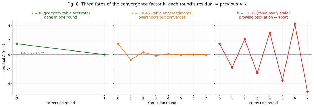
Fate 1 — k = 0: one-shot. The stored geometry equals reality; one correction lands exactly.

Fate 2 — 0 < |k| < 1: convergence, over several rounds. Two distinct looks. Positive k (D_assumed > D_true, overestimate): each round under-corrects, residual shrinks monotonically — k = 0.6 needs 8 rounds. Negative k (D_assumed < D_true, underestimate): each round overshoots, the residual flips sign and shrinks while swinging — k = −0.46 needs 6 rounds.

That sign flip deserves a slower look, because it is genuinely counterintuitive: why does overshooting mean the next correction goes the other way? Multiplying by a negative number does two things at once — flips across zero, and scales (Figure 9):

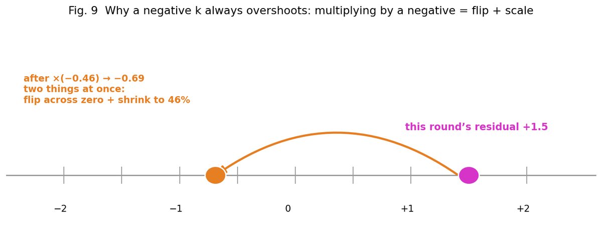
Walking the running example round by round, every multiplication shown:

So when you see a press “hunting” left-right around the target with shrinking swings, that’s not a fault — that is k = −0.46 doing its job.

Fate 3 — divergence. Since D_true ÷ D_assumed is always positive, k is always below 1, so the under-correcting type (positive k) always gets there eventually, however slowly. The danger lives at the other end: when the true lever arm reaches twice the stored value or more (k ≤ −1), the residual stops shrinking and starts growing. The only sane response is to abort and alarm — and the most common root cause is exactly this: a camera or pivot was moved, and the stored geometry no longer matches physics.

Why Optimization = Driving k Toward 0

Each round costs real time: move, settle, photograph, process, compute — roughly 2–4 seconds. k = 0.6 means 8 rounds, twenty-plus seconds per sheet; k = 0 means one round. Across thousands of sheets a day, the gap is measured in hours (Figure 10):

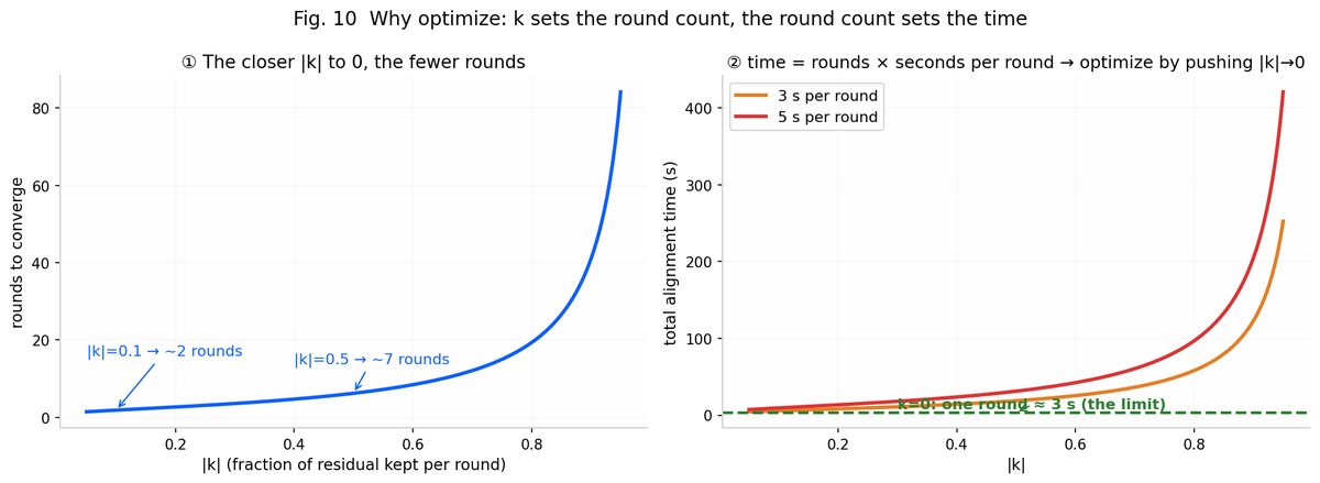
And driving k toward 0 means exactly one thing: making D_assumed equal D_true. Which raises the practical question — how do you find D_true when the cameras are buried under the table where no ruler reaches? You let the machine weigh it out itself (Figure 11):

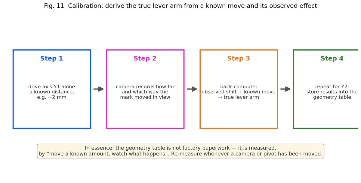
With the numbers shown: D_true = 300 × (2.92 ÷ 2.00) = 438.6 mm. Write 438.6 in place of 300, and the next alignment run is a one-shot. That is the entire essence of calibration: one known input plus one precise observation, and the model parameter snaps into agreement with reality. (This note only covers the geometry side; the pixel-to-millimeter side of calibration gets its own unit — that’s A4.)

Try It Yourself

The full lab is embedded below — the same math as this note, character for character, with nothing simplified away. Suggested path:

1. Press Y1＋ (2 mm step) and read the live calculation panel: θ, sin θ, cos θ, the full rotation-plus-translate substitution, and which-minus-which for Δ. This is Concept 3 with real numbers.
2. Press Start alignment with defaults (D_assumed 400, true distance shown above it) and read the round-by-round log.
3. Drag camera K1 to a new spot (a changeover!), then run alignment again with the stale D — watch it overshoot and oscillate; that’s Figure 9 happening live.
4. Press Run calibration — the machine measures D itself — then align again: one round, done. That’s Figure 11.
5. For the brave: set the assumed D below half the true distance and watch divergence force an abort.

The Full view button expands the lab to fill your screen — much more comfortable on a phone.

Terms in This Note

• Pivot — the point where a motor axis pushes the table; constrained to its axis line.
• Center of rotation — the one point that doesn’t move during a rotation; the pivot midpoint in the symmetric case.
• Lever arm (r) — in-plane distance from the camera’s aim point to the center of rotation; converts angles into displacements (θ × r).
• Table vs. world coordinates — the ruler nailed to the table vs. the ruler nailed to the frame; the rotation-plus-translation transform connects them.
• Deviation Δ — actual position minus target position, component by component.
• Tolerance ε — the pass line (typ. ±0.02 mm); inside it, alignment is declared done.
• Convergence factor k — 1 − D_true ÷ D_assumed; the residual’s survival ratio per round. k = 0 one-shots, |k| < 1 converges, k ≤ −1 diverges.
• Calibration — one known move plus one precise observation, used to rewrite the stored geometry so it matches physics again.

In A4 we finally get to calibration proper: how the machine learns what one pixel means in millimeters, and what a measurement run actually does.